Overview
A transformer is a neural network architecture capable of efficiently forming relationships in sequential data. It does this using a mechanism called attention.
When processing some token, attention allows the model to consider how that token is affected by all other tokens in the model's context.
Language tasks are inherently sequential, yet often depend on relationships between distant pieces of text, making them a strong use case for leveraging the attention mechanism.
Consider the following text streams:
"The capital of France is"
In this simple example, attention increases the weight of capital, France, and is to provide a higher likelihood of Paris being generated.
"def scale(values, factor):
    return [v * factor for v in"
In code generation, attention helps connect back to earlier code context. In this case, the relationship between v, the loop structure, and the input values.
Before Attention
Before attention, models often relied on long chains of memory to pass information from earlier tokens to later ones. This is the core idea behind recurrent neural networks, where information is carried forward step by step through the sequence using hidden layers (h).

It can be seen that in the unrolled recurrent neural network architecture, information must travel through potentially many hidden states which can result in dilution.
An example that highlights the problem more clearly:
The capital of France, which I visited after spending three weeks traveling through Europe and reading about its history, is
In this case, the model needs to preserve the relevance of France across many intermediate hidden states as all of the subsequent words get processed through the network.
As information is passed step by step, that signal weakens, making it difficult to encode the importance of that token. In turn, the model's prediction could become inaccurate - or, not as accurate as it would be if it maintained that relevance.
Mathematically, the information at time \(t\) is a function of the summary of the past stored in \(h_{t-1}\), combined with the current input \(x_t\).
With Attention
With attention, the current position does not need to rely on many sequential recurrent steps and can instead directly read from earlier relevant positions.
The representation of position t is the weighted sum of all of the value vectors from all positions j:
If token \(t\) needs information from token \(j\), it does not need to preserve that signal through \(t-j\) recurrent transitions. It can form a direct weighted connection to that earlier token.
The attention mechanism removes the need for serial information to "survive" long chains by allowing each token to access the information of all other tokens in the current context. The impact of past tokens is no longer a function of their values and their signal strength as they pass through the network, but merely a function of their values. As a result of this, deep dependencies are easier to learn and can more effectively be used to generate more probable output.
This is the key breakthrough that introduced the transformer architecture as an effective means of sequence modeling in Attention Is All You Need.[1]
Backpropagation and Vanishing Gradient in Recurrent Neural Networks
Along with information loss through the network, sequential depth in recurrent neural networks also makes training harder because it leads to the vanishing gradient problem.
The most common way neural networks are trained is using backpropagation.
At a high level, it determines how the error (loss function) is affected by the currently layer's outputs which, in turn, is a function of the previous layer's outputs and model weights, recursively. It then updates the weights to minimize the error loss for the next iteration.
Mathematically, \(h^{(l)}\), the output of layer \(l\), is a function of the output of layer \(l-1\) and the weights at layer \(l\), \(W^{(l)}\).
Computing the gradients determines how each layer (and therefore weight) affects the error.
From there, the weights are updated to minimize the error for the next pass. This continues to occur via billions/trillions of cycles on diverse inputs, resulting in the final weights and biases matrices that a model gets shipped with.
The vanishing gradient problem describes the behavior where, as backpropagation moves toward earlier layers of a neural network, the gradient becomes so small that the influence of those layers on the loss effectively vanishes. This typically occurs because the gradient is repeatedly multiplied by values whose magnitudes are less than 1, causing it to shrink exponentially.
Recurrent neural networks are prone to this behavior because expanding their recurrence relation (unrolling) reveals that the gradient at early timesteps is a long product of repeated transformations with common factors.
During backpropogation, the partial derivative of the loss function with respect so some hidden layer timestep becomes a massive product of partial derivatives by the chain rule. However, from the recurrence relation above, it becomes apparent that each the partial derivatives contain common factors (namely, W_hh) which, in turn, are repeatedly multiplied throughout. If these common terms are less than 1, the gradient diminishes.
Phrased differently, because the same \(W_{hh}\) appears at every step of the recurrence, it also appears repeatedly in the backward pass. At each timestep, the gradient is multiplied by a factor involving both the recurrent weight \(W_{hh}\) and the slope of the activation function at that step, \(f'(a_i)\), where \(a_i = W_{hh}h_{i-1} + W_{xh}x_i + b\). If these repeated factors tend to be smaller than \(1\) in magnitude, their product shrinks rapidly over many timesteps. As a result, early hidden states contribute very little to \(\frac{\partial L}{\partial h_i}\), and therefore also very little to \(\frac{\partial L}{\partial W_{hh}}\).

If early timesteps contribute only very small gradients, then the total gradient is dominated more by recent timesteps than by long-range dependencies. In that case, information from earlier parts of the sequence has very little effect on the update, so those contributions are effectively lost. In the context of sequential processing of information, this is undesireable since signfiicant meaning from words/data at the beginning of the processing chain can be lost, preventing accurate understanding of the remaining data's context.
In a transformer architecture with attention layers, the impact of these long-range dependencies is less likely to be lost during training because each token can attend directly to relevant earlier tokens, rather than forcing information and gradients to pass through a long chain of recurrent steps.
Transformer Architecture
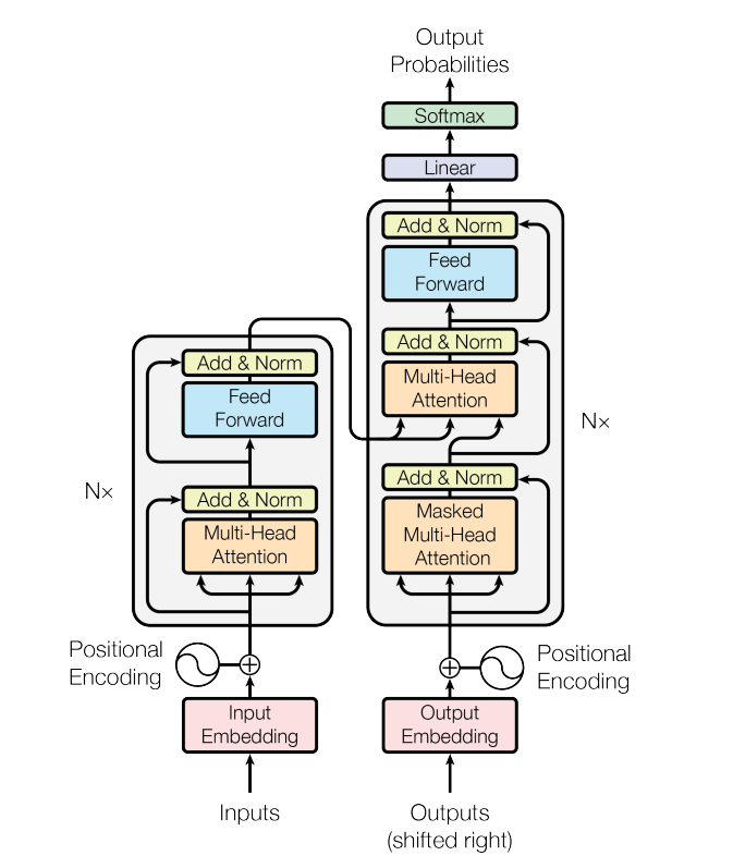
The transformer architecture replaces recurrence with stacked attention and feedforward blocks, allowing each token to gather context from the entire sequence in parallel.
Encoder models receive an input and build a representation of it. They are useful when the goal is to understand the input, such as in sentence classification or entity recognition. BERT is a common example.
Decoder models generate a sequence one token at a time using prior context. They are useful for generative tasks such as text generation. GPT is a common example.
Encoder-Decoder models use the encoder to understand the input and the decoder to generate the output. They are useful for tasks such as translation and summarization. T5 and the original transformer are common examples.
Decoder Flow
1. Token Embeddings and Positions
Raw tokens are encoded into some N-dimensional vector. Positional information is encoded as well.

2. Masked Self-Attention
After getting encoded into some high-dimensional vector representation of real numbers, the token being processed heads to the attention layers.
There are 3 different projected representations used in attention:
- Query (Q) which determines what kind of information the current position wants to retrieve
- Key (K) which is compared against queries to decide how relevant each token is
- Value (V) which is the information mixed into the output according to those attention weights


For a decoder architecture, the current token being processed should only have context of all previously processed tokens to that point. This is reffered to as its autoregressive property. Therefore future tokens are masked with negative infinity which become zero following softmax.
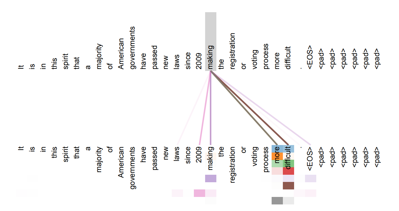
Now the updated France vector carries not just "France-ness", but a more contextual representation relating France to the concept of a capital in a city. This helps the decoder provide a more accurate prediction for the next appropriate token.
In another example:
"The snack-seeking, scruffy dog ran to the"
dog changes as adjectives add context.
Attention helps the model treat dog in the context of the full phrase, not just as an isolated word. As described earlier, the updated encoding (directionality of dog) is a function of the updated score matrix that that "embeds" the adjective information into the "dog" information.
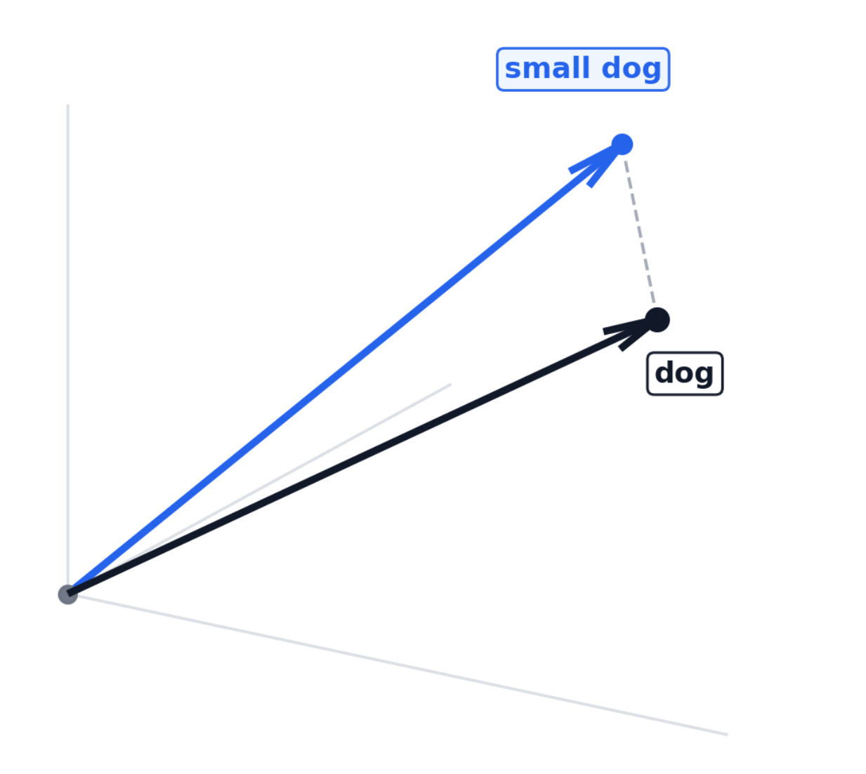
In an oversimplified mental picture, different "directions" in the hyper-dimensional space can represent different meanings. In 3 dimensions - one dimension can represent "dog-like" qualities, one can represent "scruffy-like" qualities, and one can represent "snack-seeking-like" qualities...
The "dog" vector now reflects the full phrase instead of the word alone. The model is then more likely to predict a location where a snack-seeking, scruffy dog would run to...
3. Feedforward Layer and Next-Token Prediction
The transformer also has feedforward elements. These are no different than a traditional feedforward neural network. They have their own weights and discover some kind of other useful meaning. This is a high level description with lots of potential for deep dives...
By the end of these serial layers, the transformer takes the last hidden vector h and
multiplies it by a vocabulary matrix. This produces one raw score for every possible token in the
vocabulary.
These are not probabilities yet. They are just raw scores, so for a phrase like
The capital of France is, the model might assign larger values to more plausible next
tokens.
"Paris"   -> 12.3
"London"  -> 4.8
"city"    -> 3.1
"banana"  -> -2.0
Softmax then turns those logits into probabilities:
After softmax, the model now has a probability distribution over the vocabulary:
"Paris"   -> 0.82
"London"  -> 0.06
"city"    -> 0.03
...
The decoder can then choose the next token from this distribution. It may do this using many heuristics on top of the probability. For example, it may manage repetition by adding presence or frequency penalties that help keep the model from repeating itself. Likewise, limits on total token output length could exist that steer the model away from generating massive streams.
Following the generation of the next word, that word is added back into the model. Effectively, the model shifts forward, incorporating that token into the context for its next step. At this point, the model is already pre-filled with context, so re-feeding the entire input from scratch would be inefficient. To avoid this, caching is often used. The K-V vectors are kept in memory, which significantly reduces computation and speeds up future passes through the model.
The Trade With More Context
More context allows the model to look back at more information that's hopefully relevant. That information can provide deeper insight for more accurate generation. However, as the context grows, attention layers become more expensive in both compute and memory. Q, K, and V grow with n, while the attention value matrix grows with n^2.
If K-V caching is implemented, a larger context also increases the amount of memory needed during execution steps of the model.
Tokenization
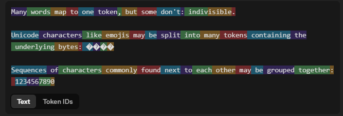
Tokenization refers to the way input is partitioned into units, which are called tokens. There are many ways that words can be partitioned or tokenized. While larger tokens require less computation resources (since more information is grouped together), they also require more memory (since more "unique information" needs to be encoded rather than relying on smaller subset chunks). Larger tokens may also not work well with typos since they may rely on exact word representations.
Byte pair encoding is one popular encoding method. It merges commonly present byte pairs together as the basis for tokens. It's not as verbose as having all characters be unique tokens (which results in massive amounts of data) but also more flexible than having tokens be words.
Embeddings
After being tokenized, the tokens are mapped to a high-dimensional vector that "aquire meaning" throughout the transormer process to end up forming a probability distribution of the next most likely tokens. The tokens get corresponding token ids that map to the embedding lookup.
tokens     -> ["small", "dog"]
token IDs  -> [1834, 481]
lookup     -> [E[1834], E[481]]
As mentioned earlier, the vectors encode infromation. One way to think of it is that the vector encodes multi-dimentional directions, with each direction representing some piece of "meaning". An oversimplified 3D visual can help illustrate the point:
The embedding lookup gives the model an initial vector. Attention layers, described earlier, can update that vector using context and shift it toward a more specific meaning.
Optimization
Inference-Time Optimization
Inference-time optimizations refer to optimizations that improve performance at the time of model execution. Performance can be quantified in various different ways including the latency from input to first token generated, the amount of memory used, the amount of compute used, etc etc.
This can be its own post (or multiple) so keeping things at a high level, some of the largest low-hanging fruit optimizations include:
- Caching intermediate model representations (KV)
- Quantizing weights and activations
- Quantizing embeddings
Caching
Transformer models have learned parameters, which are obtained during training and remain fixed at inference time. They also have input-dependent activations, which vary as a function of the input passed into the model. Examples of learned parameters include the query, key, and value weight matrices \(W_Q\), \(W_K\), and \(W_V\). But the \(Q\), \(K\), and \(V\) matrices, which are functions of both the input and those learned weights, such as \(Q = XW_Q\), depend on all of the input the model has processed so far during inference.
As new input is fed into the model, it would be very wasteful to have to recompute those internal intererence-time states. That would significantly increase compute and add lots of latency. Instead of doing that, those runtime parameters can be cached such that by processing the next token, the model builds upon the previous representations instead of recomputing them entirely. This trades compute and latency for memory, so it's often critical to strike a balance with the amount of context that the model can accept.
An extreme example helps illustrate the value of inference-time caching. Suppose a model is given a 100-page PDF and asked to first identify its main topics. Without caching, every newly generated token would require the model to repeatedly recompute representations for the entire document. With caching, those earlier computations can be reused, allowing the model to focus only on the newly generated token while still referencing the full prior context. Subsequent queries to then summarize the pdf or determine its tone are able to run much faster since the "representation" of the PDF is maintained.
Quantization
Quantizing refers to the process of converting numerical data to lower precision via a lower-capacity data type.
In the example above, the original weight matrix may have needed 32 bits per weight (f32) wheras the quantized representation may only need 8 bits per weight (int8) with a scalar that allows the matrix to get dequantized.
float32 weight: 0.1827364   # stored in 32 bits
int8 weight:    18          # stored in 8 bits
scale:          0.01

approx value = 18 * 0.01 = 0.18
Applying this back to the transformer model -- quantization can result in massive decreases in memory and increases in speed at the trade of accuracy.
As mentioned earlier, there are billions of parameters that are stored and used in computations through the transformer.
These need to be pulled into GPU memory, transferred around, and used for arithmetic constantly. By quantizing these values, the shapes of the learned parameter matrices such as W_Q, W_K, W_V, W_O, and the feedforward weights W_1 and W_2 remain the same, but their stored size footprints drop. Intermediate calculations that depend on those quantized values can also become cheaper.
It's also possible to quantize the embeddings (high-dimentional vector representations of tokens). This, in turn, reduces the dimensionionality of many of the arithmentic operations that occur thoughout the transformer (matrix multiplies, maxtrix by scalar multiplies, etc). Reduced dimensionality of arithmetic reduces the compute required to perform it and memory footprint. There is a whole field of research dedicated to dimensionality reduction while still maintaining precision.
There are also efforts to reduce quantization overhead (like the scale factor mentioned in the quantization example above). On March 24, 2026, Google Research introduced TurboQuant and PolarQuant as approaches for reducing quantization overhead via more compact ways of encoding the information needed to perform dequantization.[7]
References
- [1] Google: Attention Is All You Need
- [2] Attention in transformers, step-by-step | Deep Learning Chapter 6
- [3] Hugging Face LLM Course
- [4] SuperDataScience: recurrent neural networks and the vanishing gradient problem
- [5] OpenAI: Improving Language Understanding by Generative Pre-Training
- [6] NVIDIA Technical Blog: Optimizing LLMs for Performance and Accuracy with Post-Training Quantization
- [7] Google Research Blog: TurboQuant: Redefining AI efficiency with extreme compression
- [8] Microsoft Learn: Understanding tokens
- [9] OpenAI: Tokenizer